R&D Projects
Simulation-Based Prediction of Sleep Apnea
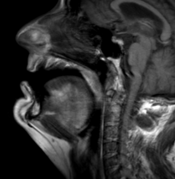
Fig 1. MRI scan depicting the upper airway of a patient diagnosed with severe Obstructive Sleep Apnea (OSA).
The initial and critical step for a Computational Fluid Dynamics (CFD) project on sleep apnea is the Magnetic Resonance Imaging (MRI) image acquisition. This involves capturing a series of high-resolution, cross-sectional images of a patient’s upper airway (including the nasal passages, pharynx, soft palate, and tongue). MRI is particularly advantageous over other imaging modalities like CT because it offers superior soft-tissue contrast, which is essential for clearly delineating the airway’s collapsible structures -the primary contributors to obstructive sleep apnea (OSA). Depending on the project goal, a static MRI (e.g., at end-exhalation) may be used to capture the detailed resting anatomy, or a dynamic “cine” MRI sequence may be used to capture the airway’s motion throughout a breathing cycle. These DICOM-formatted image slices serve as the foundational dataset, providing the precise, patient-specific anatomical boundaries required for the subsequent 3D model reconstruction and CFD simulation.
Following the MRI acquisition, the next step is to create a patient-specific 3D model of the upper airway lumen from the collected image stack. This process, known as segmentation, involves using specialized medical image processing software (like MIMICS or 3D Slicer) to manually or semi-automatically trace the boundary between the air column (the airway lumen) and the surrounding soft tissues (e.g., the tongue, soft palate, pharyngeal walls) on each 2D image slice. The excellent soft-tissue contrast from the MRI is crucial here for accurate boundary detection. Once all slices are segmented, the software then interpolates and stitches the 2D contours together to generate a continuous 3D surface model of the airway, typically exported as a triangulated surface file (like an STL or IGS). This 3D surface represents the computational domain – the internal volume where the air flow physics will be simulated – and its geometric accuracy directly determines the fidelity of the final CFD results for predicting sleep apnea-related airflow characteristics.
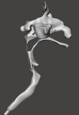
Fig 2. Three-dimensional reconstruction of the patient’s upper airway derived from MRI scans acquired in the supine position.
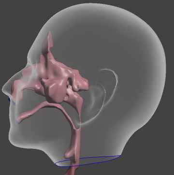
Fig 3. Schematic illustration showing the approximate location of the upper airway within the human head.
CFD Governing Equations and Solution Setup
Once you have your patient-specific 3D geometry and the flow rate boundary conditions from the sleep study, you must define the fluid mechanics and the mathematical models the CFD software will use.
1. Governing Equations
The flow of air in the upper airway is governed by the conservation laws of physics, known as the Navier-Stokes Equations (for momentum) and the conservation of mass.
Assumption: Steady-State vs. Transient (Unsteady)
Steady-State: This is the simplest approach, which is often used. It models the flow at a single, peak flow rate (e.g., peak inhalation) derived from the sleep study. It assumes the flow is constant over time, which saves computational resources.
Transient (Unsteady): This is more accurate but far more complex. It uses the entire flow waveform (the cycle of inhalation and exhalation) from the sleep study as a time-dependent boundary condition. For a WordPress tutorial, sticking to Steady-State for a specific peak flow is usually sufficient for demonstration.
2. Turbulence Model Selection
Airflow within the constricted and irregular geometry of an obstructed airway, as encountered in Obstructive Sleep Apnea (OSA), is predominantly turbulent or transitional in nature. Accurate representation of this phenomenon necessitates mathematical modeling. The table below summarizes selected numerical models and provides recommendations for identifying the most appropriate approach for this application.
Model | Description | Recommendation for Airway Flow |
Laminar Flow | Assumes smooth, orderly flow. Only suitable for very low, resting breathing rates. | Not recommended for peak flow or OSA. |
k-ω SST (Shear Stress Transport) | A robust Reynolds-Averaged Navier-Stokes (RANS) model. It is excellent for capturing flow separation and near-wall effects, which are critical at the narrowest parts of the airway. | Best Practice for initial, steady-state OSA simulations due to good accuracy and reasonable computational cost. |
Standard k-ϵ | A less accurate RANS model near walls. | Generally less accurate for upper airway flows than k-ω SST. |
LES (Large Eddy Simulation) | The most accurate model for unsteady, turbulent flow, but requires massive computing power. | Reserved for advanced, transient analysis. |
Recommended Choice: Use the k-ω SST turbulence model. You will need to set the Turbulence Intensity at your velocity inlet/outlet boundary, often a nominal value of 5% to 10%.
3. Solver and Convergence Settings
These settings tell the software how to solve the equations and when to stop the calculation.
Solver Type: Pressure-based solver is standard for low-speed, incompressible flow like respiration.
Discretization Schemes: Use Second-Order Upwind schemes for momentum, turbulence, and energy (if including heat transfer). This balances accuracy with stability.
Convergence Criteria (Residuals): The simulation stops when the solution is stable, which is measured by residuals (a measure of error). The convergence target should be set to a low value: 10−4 or 10−5 for the velocity and turbulence residuals, and 10−6 for the continuity (mass) residual.
4. Key Results to Extract
The entire purpose of the CFD is to calculate fluid flow metrics that relate back to the patient’s condition. The most important results to extract are:
Minimum Airway Wall Pressure (Pmin): The lowest pressure value on the inner surface of the airway wall. A very low (highly negative) pressure indicates a high risk of the airway walls collapsing, which is the mechanism of obstructive apnea.
Flow Resistance (R): Calculated as the pressure drop (ΔP) between two points (e.g., nose and trachea) divided by the flow rate (Q):
R=ΔP/Q
A high resistance value is a direct measure of airway obstruction.
Velocity Magnitude and Jetting: High-velocity jets of air form just downstream of the narrowest part of the airway. Visualizing this jet helps pinpoint the precise location and severity of the collapse.
Turbulent Kinetic Energy (TKE): This quantifies the intensity of turbulence. High TKE is often associated with the site of obstruction and a source of loud snoring or flow limitation.
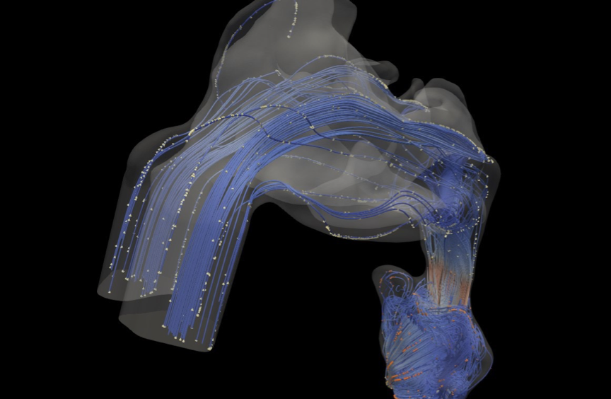
Fig 4. CFD simulation results illustrating velocity streamlines and dispersed particles at various sections of the upper airway.
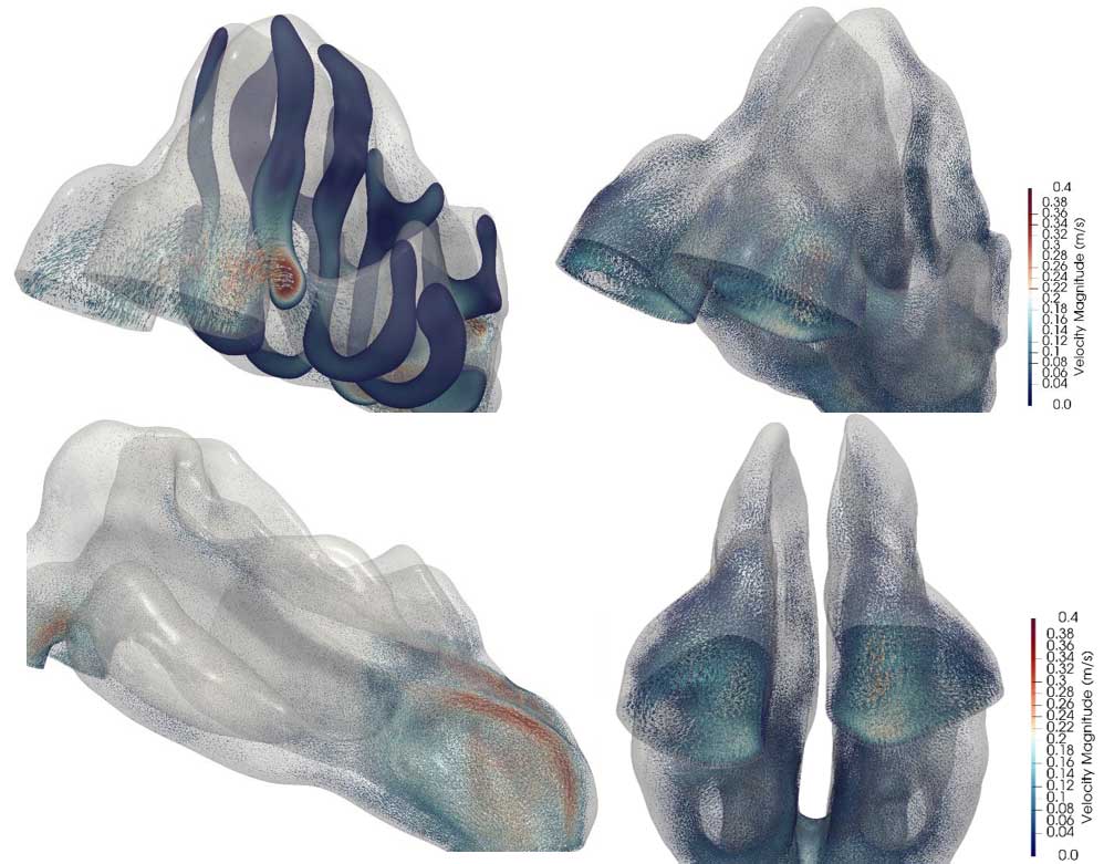
Fig 5. CFD results illustrating the velocity magnitude within the upper airway during inhalation, presented from multiple views.
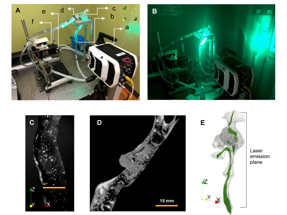
Fig 6. Experimental PTV setup for the rigid and semi-flexible laboratory airway models. (a) Phantom high-speed camera. (b) The outlet of the rigid model was carefully sealed at the bottom of the trachea. (c) The orientation of the rigid model, which replicates the seating position of the subject. (d) Pipes carefully attached and sealed to nostrils. (e) SuperPump driving cyclic breathing with a sinusoidal volumetric flow (amplitude 32.1 cm3 /s). (f) Location of light source (530 nm, 80 mW, 12 V) for laser sheet’. (B) Moment of laser emission and PTV photography (no ambient light). (C) Trachea region during inhalation at 0.47 s after inhalation with particles fluorescing in the laser light (yellow line represents the reference length scale). (D) Pharynx region at 0.47 s after the commencement of inhalation. (E) Location of the laser sheet along the upper airway
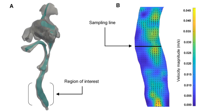
Fig 7. (A) Geometry of the patient’s upper airway model that was used for the particle tracking study. This includes slice-like subdomain illuminated by the laser sheet (depicted in green). (B) Experimentally measured velocity field within the slice and region of interest (trachea) at time 0.47 s (U = 65) during the inhalation cycle. The velocity distribution along the sampling line is used here as a basis for validating the numerical model.
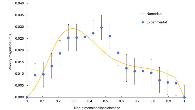
Fig 8. Comparison of the experimental and numerical velocity profiles along the sampling line shown in Fig. A1(B) at time 0.47 s (U = 65) during the inhalation cycle. The orange line represents the numerical velocity profile scaled by the kinematic viscosity ratio for air and water (a = 14). The blue points indicate the experimentally measured velocity profile (averaged over eight flow cycles) with the error bars representing the total uncertainty, which includes both the standard deviation in the velocity magnitude data and the systematic uncertainty associated with the laser sheet’s finite thickness.
For further details, please refer to the full published paper available via the link below.
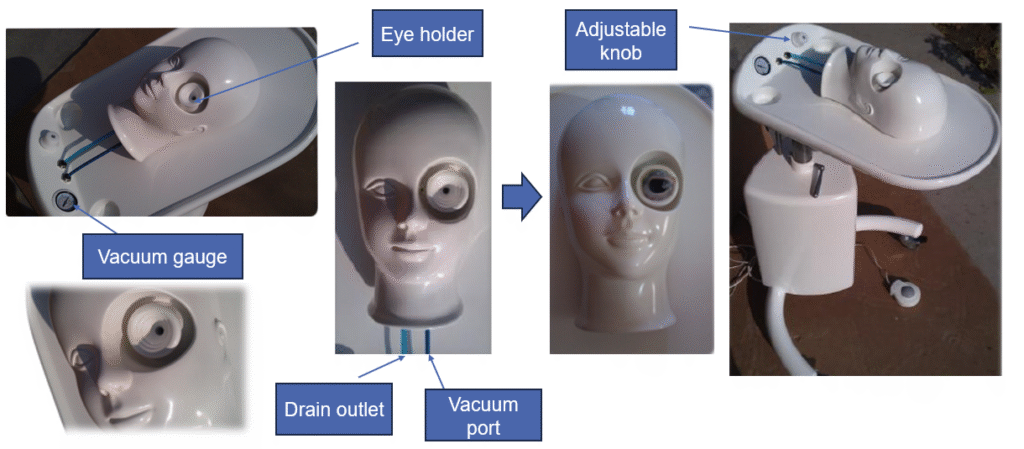
Innovative Globe-Fixation System for Ophthalmic Surgical Training